ダイクストラ法

ダイクストラ法をRとigraphを使って表現する．

igraphのshortest.paths関数で一発でできるのだけど，お勉強のためということで．

まずは最短経路を求めるグラフを用意する．

library(igraph)
g<-graph.empty(5)
V(g)$name<-c("A","B","C","D","E")
g<-add.edges(g,c(0,1,0,2,0,3,1,2,1,3,1,4,2,3,3,4))
g<-as.undirected(g)
E(g)$weight<-c(2,1,7,5,6,1,1,8)
lay<-rbind(c(1,3),c(2,3),c(1,1),c(2,1),c(3,2))
plot(g, layout=lay,vertex.label=V(g)$name,vertex.size=12,edge.label=E(g)$weight)

こんな感じ．今回はノード「E」をゴールとする．

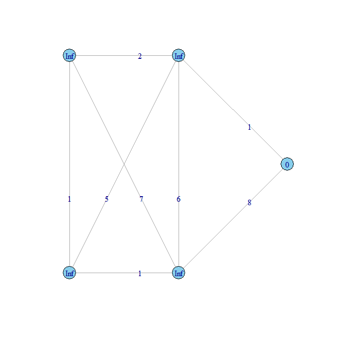
つぎに各ノードのコストを初期化する．

V(g)$cost<-c(Inf,Inf,Inf,Inf,0)
V(g)$fixed=FALSE
V(g)$color<-"skyblue"
plot(g, layout=lay,vertex.label=V(g)$cost,vertex.size=12,edge.label=E(g)$weight,vertex.color=V(g)$color)

つぎはコスト計算．

V(g)[nei(V(g)[fixed==FALSE & cost==min(V(g)[fixed==FALSE]$cost)]) & fixed==FALSE][V(g)[nei(V(g)[fixed==FALSE & cost==min(V(g)[fixed==FALSE]$cost)]) & fixed==FALSE]$cost>(E(g)[V(g)[fixed==FALSE] %->% V(g)[fixed==FALSE & cost==min(V(g)[fixed==FALSE]$cost)]]$weight)+(V(g)[fixed==FALSE & cost==min(V(g)[fixed==FALSE]$cost)]$cost)]$cost<-(E(g)[V(g)[fixed==FALSE] %->% V(g)[fixed==FALSE & cost==min(V(g)[fixed==FALSE]$cost)]]$weight)+(V(g)[fixed==FALSE & cost==min(V(g)[fixed==FALSE]$cost)]$cost)

ながい．．．もっと短くできるかもしれない．

V(g)[fixed==FALSE & cost==min(V(g)[fixed==FALSE]$cost)]$color="yellow"
V(g)[fixed==FALSE & cost==min(V(g)[fixed==FALSE]$cost)]$fixed=TRUE

計算が終わったノードは黄色に塗りつぶす．

plot(g, layout=lay,vertex.label=V(g)$cost,vertex.size=12,edge.label=E(g)$weight,vertex.color=V(g)$color)

これを計算するノードが無くなるまで繰り返す．

もう一回．

もう一回．

もう一回．

もう一回．

これで終わり．

実際にグラフを描きながらだと楽しいね．

R + igraph + Cytoscape

まずはR+igraphでネットワークグラフを作成する．

> library(igraph)
> d<-matrix(c(0,0,1,1,1 ,0,1,1,0,2,0,3,1,0,1,6,0,0,0,2,1,8,5,2,0),ncol=5,nrow=5)
> ls()
[1] "d"
> d
     [,1] [,2] [,3] [,4] [,5]
[1,]    0    0    0    6    1
[2,]    0    1    3    0    8
[3,]    1    1    1    0    5
[4,]    1    0    0    0    2
[5,]    1    2    1    2    0
> g<-graph.adjacency(d,weighted=TRUE)
> summary(g)
Vertices: 5
Edges: 15
Directed: TRUE
No graph attributes.
No vertex attributes.
Edge attributes: weight.
> degree(g)
[1] 5 6 7 4 8
> png("c:/tmp/myplot.png",width=600, height=600,pointsize=14)
> plot(g,layout=layout.fruchterman.reingold,vertex.label=V(g)$smr,vertex.size=degree(g)*4)
> dev.off()
null device
          1

なかなか，いい感じ．

つぎはCytoscape（http://www.cytoscape.org/)を使って描画してみる．

まずは，Rからグラフをエキスポートする．

このときファイルタイプとして”ncol”を指定するのを忘れずに！

> write.graph(g,"c:/tmp/mygraph.ncol","ncol")

Cytoscapeを起動して[File]>[Import]>[Network from Table(Text/MS Excel...)]を選択する．

先ほどエキスポートした「c:/tmp/mygraph.ncol」を読み込む．

[Source Interaction]に「Column 1」，[Interaction Type]に「Column 3」，[Target Interaction]に「Column 2」を設定する．

[Import]ボタンをクリックする．

これでグラフをインポートできた．

あとはCytoscpae上でグラフを色々と見やすくしてやればいい．

R+igraphのお勉強 その3

ノードの次数を確認する．

> g
Vertices: 10
Edges: 9
Directed: TRUE
Edges:
         
[0] 0 -> 1
[1] 0 -> 2
[2] 1 -> 3
[3] 1 -> 4
[4] 2 -> 5
[5] 2 -> 6
[6] 3 -> 7
[7] 3 -> 8
[8] 4 -> 9

次数を確認する．

> degree(g)
 [1] 2 3 3 3 2 1 1 1 1 1

入次数を確認する．

> degree(g,mode="in")
 [1] 0 1 1 1 1 1 1 1 1 1

出次数を確認する．

> degree(g,mode="out")
 [1] 2 2 2 2 1 0 0 0 0 0

 当然，無向グラフに入出の区別はない．

> g2
Vertices: 10
Edges: 9
Directed: FALSE
Edges:
         
[0] 0 -- 1
[1] 0 -- 2
[2] 1 -- 3
[3] 1 -- 4
[4] 2 -- 5
[5] 2 -- 6
[6] 3 -- 7
[7] 3 -- 8
[8] 4 -- 9

次数を確認する．

> degree(g2)
 [1] 2 3 3 3 2 1 1 1 1 1
> degree(g2)
 [1] 2 3 3 3 2 1 1 1 1 1
> degree(g2,mode="in")
 [1] 2 3 3 3 2 1 1 1 1 1
> degree(g2,mode="out")
 [1] 2 3 3 3 2 1 1 1 1 1

ノードの次数をノードのサイズに設定してグラフを描画する．

> png("plot3.png",width=400, height=400,pointsize=12)

次数の10倍をノードサイズとする．

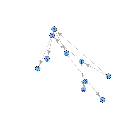
> plot(g,layout=lay,vertex.size=degree(g)*10)
> dev.off()
null device
          1

R+igraphのお勉強 その2

前回の続き．

有向グラフを無向グラフに変換してみる．

有向グラフの確認．

> is.directed(g)
[1] TRUE

無向グラフに変換する．

> g2<-as.undirected(g)

変換結果を確認する．

> g2
Vertices: 10
Edges: 9
Directed: FALSE
Edges:
         
[0] 0 -- 1
[1] 0 -- 2
[2] 1 -- 3
[3] 1 -- 4
[4] 2 -- 5
[5] 2 -- 6
[6] 3 -- 7
[7] 3 -- 8
[8] 4 -- 9
> is.directed(g2)
[1] FALSE

グラフを描画する．

> png("plot2.png",width=400, height=400,pointsize=12) 

> plot(g2,layout=lay)

> dev.off()
null device
          1

作業経過をファイル保存する．

 > save(g,g2,lay,file="test.dat")

R+igraphのお勉強 その1

igraphライブラリを読み込む．

> library(igraph)

10ノードのツリーグラフを作成する．

> g<-graph.tree(10)
> summary(g)
Vertices: 10
Edges: 9
Directed: TRUE
No graph attributes.
No vertex attributes.
No edge attributes.
> g
Vertices: 10
Edges: 9
Directed: TRUE
Edges:
         
[0] 0 -> 1
[1] 0 -> 2
[2] 1 -> 3
[3] 1 -> 4
[4] 2 -> 5
[5] 2 -> 6
[6] 3 -> 7
[7] 3 -> 8
[8] 4 -> 9

グラフをレイアウトする． 

> lay<-layout.fruchterman.reingold(g)

> lay
            [,1]       [,2]
 [1,]  0.5750165 -0.7339218
 [2,]  4.2972271 -0.9157740
 [3,] -2.8644359  0.1233019
 [4,]  5.7313203  2.7760283
 [5,]  5.3732637 -4.4586431
 [6,] -3.4715509  3.4824008
 [7,] -4.1404984 -2.9629157
 [8,]  4.2804038  5.9832150
 [9,]  8.9190178  2.4068283
[10,]  4.1109849 -7.2698722

 ここまでの作業をファイル保存する．

> save(g,lay,file="test.dat")

グラフを描画する．

> plot(g,layout=lay)
> png("plot.png",width=400, height=400,pointsize=12)
> plot(g,layout=lay)
> dev.off()
null device
          1

グラフレイアウト

とりあえずライブラリをロードする．

> library(igraph)

とりあえずツリーグラフを作成する．

> g<-graph.tree(4)
> plot.igraph(g)

グラフをレイアウトする．

> lay<-layout.kamada.kawai(g)
> lay
             [,1]       [,2]
 [1,] -1.95786789 -0.6726298
 [2,] -0.97281249 -1.2272012
 [3,] -2.94060962 -0.1762201
 [4,]  0.09102538 -0.7586657
 [5,] -1.03996471 -2.3633110
 [6,] -3.22145269  0.8896139
 [7,] -3.96005388 -0.5896342
 [8,]  0.59269741  0.2250630
 [9,]  1.10354845 -1.2044752
[10,] -1.05079882 -3.4245322

再描画．

> plot.igraph(g,layout=lay)

ちゃんとレイアウトされた．

Rでネットワーク図を描く3

 今度は行ラベル，列ラベルを付けてみる．

> d<-matrix(c(0,0,1,1,1 ,0,1,1,0,2,0,3,1,0,1,6,0,0,0,2,1,8,5,2,0),ncol=5,nrow=5
> d
     [,1] [,2] [,3] [,4] [,5]
[1,]    0    0    0    6    1
[2,]    0    1    3    0    8
[3,]    1    1    1    0    5
[4,]    1    0    0    0    2
[5,]    1    2    1    2    0

 まずは列ラベルを設定する．

> colnames(d)<-c("A","B","C","D","E")
> d
     A B C D E
[1,] 0 0 0 6 1
[2,] 0 1 3 0 8
[3,] 1 1 1 0 5
[4,] 1 0 0 0 2
[5,] 1 2 1 2 0

お次は行ラベルを設定する．

> rownames(d)<-c("A","B","C","D","E")
> d
  A B C D E
A 0 0 0 6 1
B 0 1 3 0 8
C 1 1 1 0 5
D 1 0 0 0 2
E 1 2 1 2 0

グラフに変換する．

> g<-graph.adjacency(d,weighted=TRUE)

画像に書き出す．

> png("c:/tmp/myplot.png",width=400, height=400,pointsize=12)
> plot(g)
> dev.off()
null device
          1 

 

エッジの重みを表示する．

> E(g)$weight
 [1] 6 1 1 3 8 1 1 1 5 1 2 1 2 1 2

一応，グラフ情報もみておく．

> summary(g)
Vertices: 5
Edges: 15
Directed: TRUE
No graph attributes.
Vertex attributes: name.
Edge attributes: weight.

今度は特定のエッジを削除してみる．

重みが5以下のエッジを削除してみよう．

> g2<-delete.edges(g,E(g)[weight<=5])

グラフ情報をみると，

> summary(g2)
Vertices: 5
Edges: 2
Directed: TRUE
No graph attributes.
Vertex attributes: name.
Edge attributes: weight.

描画してみよう．

>  png("c:/tmp/myplot.png",width=400, height=400,pointsize=12)
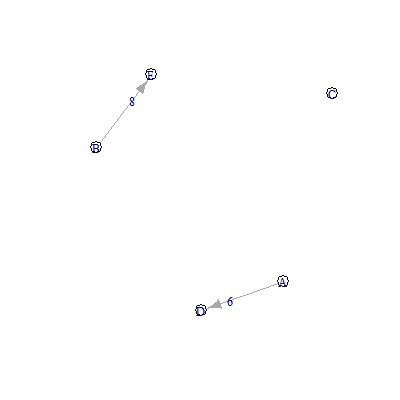
> plot(g2,layout=layout.fruchterman.reingold,vertex.color="white",vertex.label=V(g2)$name,edge.label=E(g2)$weight,vertex.size=10)
> dev.off()
null device
          1

次数0のノードができてしまった．

こいつを削除しよう．

> g2<-delete.vertices(g2,which(degree(g2)<1)-1)
> summary(g2)
Vertices: 4
Edges: 2
Directed: TRUE
No graph attributes.
Vertex attributes: name.
Edge attributes: weight.

もう一回，書き出してみる．

>  png("c:/tmp/myplot.png",width=400, height=400,pointsize=12)
> plot(g2,layout=layout.fruchterman.reingold,vertex.color="white",vertex.label=V(g2)$name,edge.label=E(g2)$weight,vertex.size=10)
> dev.off()
null device
          1

 ちゃんと削除できた．

Rでネットワーク図を描く2

こんどはもう少し大きめのグラフを書いてみる．

> library(igraph)
> d<-matrix(c(0,0,1,1,1 ,0,1,1,0,2,0,3,1,0,1,6,0,0,0,2,1,8,5,2,0),ncol=5,nrow=5
> d
     [,1] [,2] [,3] [,4] [,5]
[1,]    0    0    0    6    1
[2,]    0    1    3    0    8
[3,]    1    1    1    0    5
[4,]    1    0    0    0    2
[5,]    1    2    1    2    0
> g<-graph.adjacency(d,weighted=TRUE)
> png("c:/tmp/myplot.png",width=400, height=400,pointsize=12)
> plot(g,,layout=layout.fruchterman.reingold,vertex.color="white",vertex.label=V(g)$name,edge.color="black",edge.label=E(g)$weight,vertex.size=10)
> dev.off()
null device
          1

重みをエッジの幅に設定する．

 > E(g)$weight
 [1] 6 1 1 3 8 1 1 1 5 1 2 1 2 1 2
> E(g)$width<-E(g)$weight

美しくないのでやっぱり戻そう．

> E(g)$width<-1

Rでネットワーク図を描く

Rが面白い．簡単に色々とできてしまう．

今回はigraphライブラリでネットワーク図の作成にトライしてみる．

まずライブラリを読み込む．

> library(igraph)

つぎに隣接行列を作る．

> d<-matrix(c(0,0,1,1,0,1,1,0,0),ncol=3,nrow=3)

行列のサイズを確認する．

> dim(d)
[1] 3 3

行列を表示する．

> d
     [,1] [,2] [,3]
[1,]    0    1    1
[2,]    0    0    0
[3,]    1    1    0

 行列から重み付き有向グラフを作成する．

> g<-graph.adjacency(d,mode="directed",weighted=TRUE)

グラフ情報を確認する．

> summary(g)
Vertices: 3
Edges: 4
Directed: TRUE
No graph attributes.
No vertex attributes.
Edge attributes: weight.

最後にグラフを画像ファイルに書き出す．

> png("c:/tmp/myplot.png",width=400, height=400,pointsize=12)
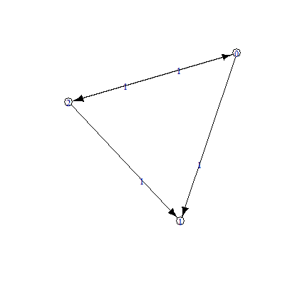
> plot(g,vertex.color="white",vertex.label=V(g)$name,edge.color="black",edge.label=E(g)$weight,vertex.size=10)
> dev.off()
null device
          1